Intro

When you have some code written in Python that is slower than you would like, you will want to make it faster. If your code spends most of its time in a big, loop, you can get more performance via Parallelism .

This post, gives some recipes on how to use the built-in concurrent.futures library to achieve parallelism.

Often, however, the performance of your code can be improved by implementing a more efficient algorithm, eliminating redundant processes or using a different function from your package — optimization.

Premature optimization is the root of all evil.
— Winston Churchill

The traditional takeaway from the above quote is that you should try to measure which parts of your code are actually slow, so you can spend your time and mental energies on where they will yield the most improvement.

So, how can you measure which parts of your code are slow?

prun in Jupyter

If you are writing code in a Jupyter notebook, you can use the prun magic command, provided by IPython.

• Apply it to a single line by prepending %prun with one %
• Apply it to the whole cell by using %%prun with two %s.

The effect of this is that when the code is executed, you will also get a ranking of the time spent in each function. You then know what to focus on to get your code running faster.

Let's give a simple and silly example.

%%prun


def sum_of_squares_slow(n):
    total = 0
    for i in range(1, n + 1):
        total += i * i
    return total


def polynomial(x):
    return x * x - 2 * x + 2


n = 1000000
x = sum_of_squares_slow(n)

y = polynomial(x)

The output looks like this:

5 function calls in 0.025 seconds

   Ordered by: internal time

   ncalls  tottime  percall  cumtime  percall filename:lineno(function)
        1    0.025    0.025    0.025    0.025 <string>:1(sum_of_squares_slow)
        1    0.000    0.000    0.025    0.025 {built-in method builtins.exec}
        1    0.000    0.000    0.000    0.000 {method 'disable' of '_lsprof.Profiler' objects}
        1    0.000    0.000    0.025    0.025 <string>:1(<module>)
        1    0.000    0.000    0.000    0.000 <string>:12(polynomial)

• tottime Time spent in the body of the function alone, not including calls to other functions. The table is sorted by this value by default.
• cumtime Time spent running the function, including its function calls.

We can clearly see that sum_of_squares_slow is slow and could be looked at, but polynomial is not a problem at this point.

timeit in Jupyter

Another useful line magic is %timeit. You can use it if you have two candidates and want to compare how long they take to run. The nice thing about timeit is it will call the function repeatedly and give you a robust average time. The slower your function, the fewer repeats, to stop you waiting so long.

def sum_of_squares_fast(n):
    return n * (n + 1) * (2 * n + 1) // 6

%timeit sum_of_squares_slow(n)
%timeit sum_of_squares_fast(n)

We see that the new fast version of the calculation is indeed much faster than the original implementation.

25.3 ms ± 249 μs per loop (mean ± std. dev. of 7 runs, 10 loops each)
81.2 ns ± 0.679 ns per loop (mean ± std. dev. of 7 runs, 10,000,000 loops each)

Note that %timeit works with any Python statement, not just function calls like in the example.

A More Realistic Example

The block below shows a function that calculates a monthly sequence of dates starting at a given date. It uses the relativedelta class from the python-dateutil library.

def month_sequence(start_month: date, n: int) -> list[date]:
    out = []
    cur_month = start_month
    for _ in range(n):
        out.append(cur_month)
        cur_month += relativedelta(months=1)
    return out

Let's use %prun to profile it.

%prun month_sequence(date(2000,1,1), 10000)

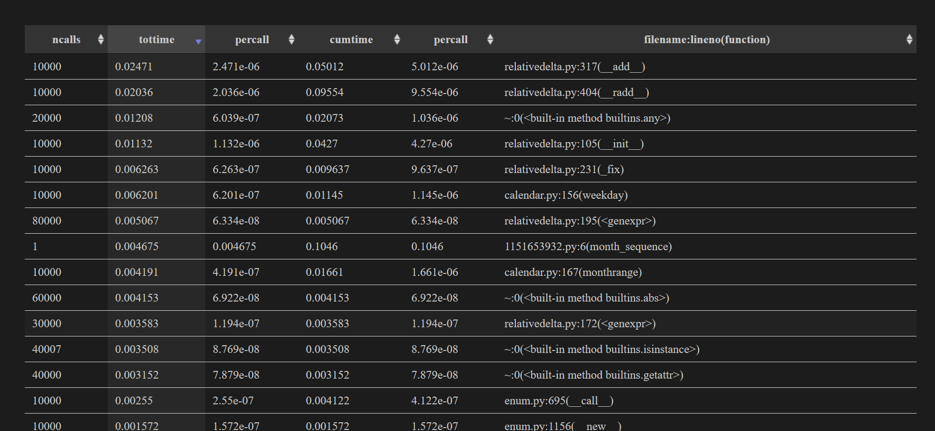
400909 function calls in 0.172 seconds

   Ordered by: internal time

   ncalls  tottime  percall  cumtime  percall filename:lineno(function)
        1    0.079    0.079    0.099    0.099 <string>:1(<module>)
    10000    0.023    0.000    0.047    0.000 relativedelta.py:317(__add__)
    20000    0.012    0.000    0.020    0.000 {built-in method builtins.any}
    10000    0.011    0.000    0.041    0.000 relativedelta.py:105(__init__)
    10000    0.006    0.000    0.011    0.000 calendar.py:156(weekday)
    10000    0.006    0.000    0.009    0.000 relativedelta.py:231(_fix)
    80000    0.005    0.000    0.005    0.000 relativedelta.py:195(<genexpr>)
    10000    0.004    0.000    0.016    0.000 calendar.py:167(monthrange)
    60000    0.004    0.000    0.004    0.000 {built-in method builtins.abs}
    30000    0.003    0.000    0.003    0.000 relativedelta.py:172(<genexpr>)
    40007    0.003    0.000    0.003    0.000 {built-in method builtins.isinstance}
    40000    0.003    0.000    0.003    0.000 {built-in method builtins.getattr}
    10000    0.002    0.000    0.049    0.000 relativedelta.py:404(__radd__)
    10000    0.002    0.000    0.004    0.000 enum.py:695(__call__)
        1    0.001    0.001    0.019    0.019 1151653932.py:6(month_sequence)
...

We can see that 0.041 seconds are spent in the __init__ method of relativedelta, and we construct a new relativedelta object in each iteration. This tells us that we can speed up the function by defining the constant relativedelta(months=1) once, and reusing it in the function.

one_month = relativedelta(months=1)


def month_sequence2(start_month: date, n: int) -> list[date]:
    out = []
    cur_month = start_month
    for _ in range(n):
        out.append(cur_month)
        cur_month += one_month
    return out

Sure enough, %timeit shows that the new function is faster.

%timeit month_sequence(date(2000,1,1), 10000)
%timeit month_sequence2(date(2000,1,1), 10000)

26.1 ms ± 403 μs per loop (mean ± std. dev. of 7 runs, 10 loops each)
15.5 ms ± 81.3 μs per loop (mean ± std. dev. of 7 runs, 100 loops each)

It's not as dramatic as the sum-squares example, but it could help!

Profiling Scripts

The equivalent of %prun for a script is the following command:

python -m cProfile script.py

Visualisation Tools

So far, we have relied on the output of the prun command. Even for simple examples, there is a lot of output, showing the times of many functions which can be hard to interpret. One way to cut through the noise is to use a visualisation tool.

The workflow is to run your profile and output a profile file, then use the visualisation tool to display the profile file. If you are using %prun, use the -D flag to output a profile file. You may also want to use the -q flag to suppress the usual prun output.

%prun -qD month.prof month_sequence(date(2000,1,1), 10000)

*** Profile stats marshalled to file 'month.prof'.

If you are using cProfile, specify the output file with the -o flag

python -m cProfile -o stats.prof script.py

Once you have your profile file, you can use a visualiser tool to inspect the profile. I use snakeviz mostly, but tuna is another alternative.

I also use uvx in the command line to invoke the visualiser.

uvx snakeviz month.prof

Snakeviz as well as tuna both launch a web server and open a browser tab for you.

You will see a graph which shows about a third of the time is spent in the __init__ method

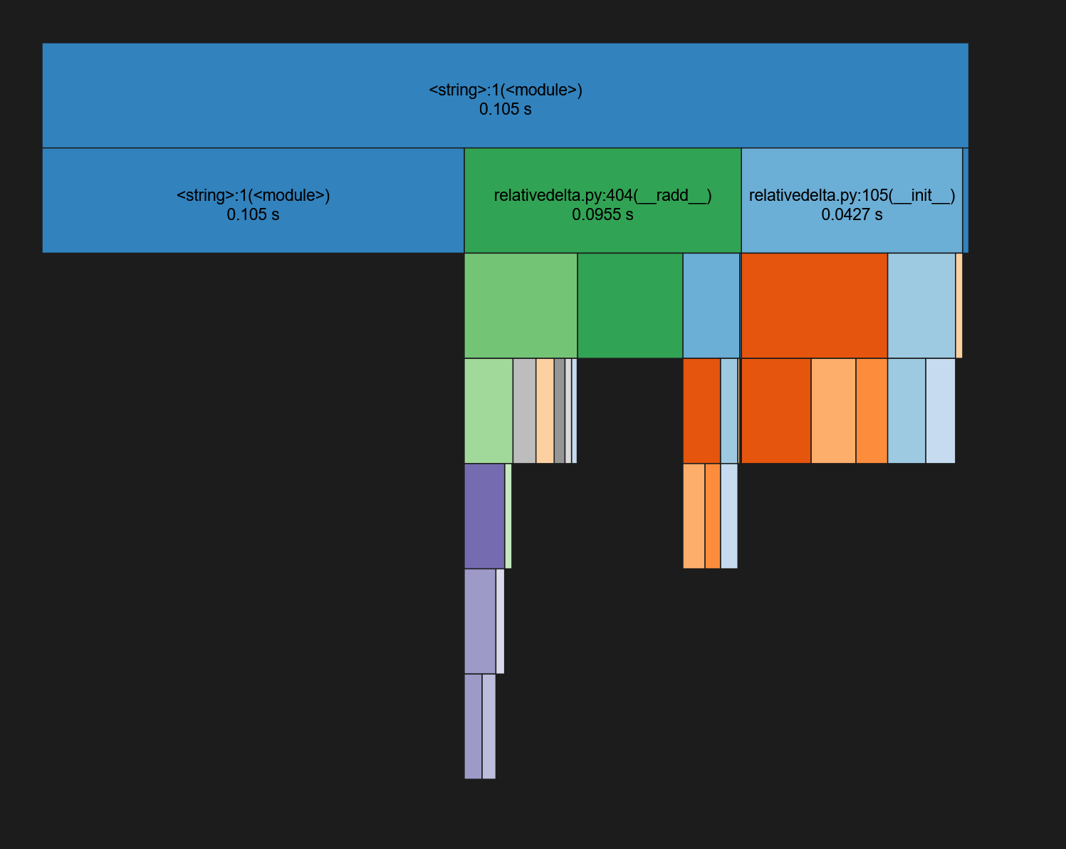
You will also see the original text information as a table, but this time you can easily sort the columns.

Profiling Multithreaded/Multiprocess Code

When the code you are trying to profile uses multiple threads or multiple processes, the profiling tools tend to give misleading or garbled information.

Instead, you can use yappi Unfortunately, you cannot run it via cell magic. The equivalent command line invocation is:

yappi -c wall -o stats.prof script.py

You can then analyse the output profile file using snakeviz or tuna.